Question

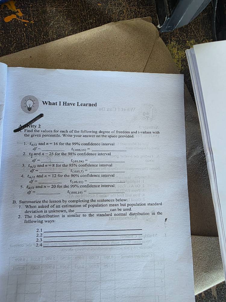
what i have learned activity 2 a. find the values for each of the following degree of freedom and t - values with the given percentile. write your answer on the space provided. 1. $t_{\alpha/2}$ and $n = 16$ for the 99% confidence interval $df = $ $t_{(0.005,15)} = $ 2. $t_{\alpha/2}$ and $n = 25$ for the 98% confidence interval $df = $ $t_{(0.01,24)} = $ 3. $t_{\alpha/2}$ and $n = 8$ for the 95% confidence interval $df = $ $t_{(0.025,7)} = $ 4. $t_{\alpha/2}$ and $n = 12$ for the 90% confidence interval $df = $ $t_{(0.05,11)} = $ 5. $t_{\alpha/2}$ and $n = 20$ for the 99% confidence interval $df = $ $t_{(0.005,19)} = $ b. summarize the lesson by completing the sentences below: 1. when asked of an estimation of population mean but population standard deviation is unknown, the \underline{\quad\quad\quad\quad} can be used. 2. the t - distribution is similar to the standard normal distribution in the following ways: 2.1 \underline{\quad\quad\quad\quad} 2.2 \underline{\quad\quad\quad\quad} 2.3 \underline{\quad\quad\quad\quad} 2.4 \underline{\quad\quad\quad\quad}

Answer:

Part A: Finding \( t_{\alpha/2} \) or \( t_{\alpha} \) values

1. \( t_{\alpha/2} \) and \( n = 16 \) for 99% confidence interval

Step 1: Calculate degrees of freedom (\( df \))

Degrees of freedom for a t - distribution when dealing with sample size \( n \) is \( df=n - 1 \). Here, \( n = 16 \), so \( df=16 - 1=15 \).

Step 2: Determine \( \alpha \) and \( \alpha/2 \)

For a 99% confidence interval, the confidence level \( CL = 0.99 \). Then \( \alpha=1 - CL=1 - 0.99 = 0.01 \), and \( \alpha/2=\frac{0.01}{2}=0.005 \).
We need to find \( t_{0.005,15} \). Using the t - distribution table or a calculator with t - distribution functionality, \( t_{0.005,15}\approx2.947 \) (from t - table: looking at the row with \( df = 15 \) and column with two - tailed \( \alpha = 0.01 \) (or one - tailed \( \alpha=0.005 \))).
So, \( df = 15 \), \( t_{(0.005,15)}\approx2.947 \)

2. \( t_{\alpha} \) and \( n = 25 \) for 98% confidence interval

Step 1: Calculate degrees of freedom (\( df \))

\( df=n - 1 \), with \( n = 25 \), so \( df = 25-1 = 24 \).

Step 2: Determine \( \alpha \)

For a 98% confidence interval, \( CL = 0.98 \), so \( \alpha=1 - 0.98 = 0.02 \). We need to find \( t_{0.02,24} \) (since it's a one - tailed test for \( t_{\alpha} \), or two - tailed with \( \alpha = 0.02 \) total, but here we are looking for \( t_{\alpha} \) so one - tailed). Using the t - table, \( t_{0.02,24}\approx2.177 \) (looking at row \( df = 24 \), column one - tailed \( \alpha=0.02 \)).
So, \( df = 24 \), \( t_{(0.02,24)}\approx2.177 \)

3. \( t_{\alpha/2} \) and \( n = 8 \) for 95% confidence interval

Step 1: Calculate degrees of freedom (\( df \))

\( df=n - 1 \), \( n = 8 \), so \( df=8 - 1 = 7 \).

Step 2: Determine \( \alpha \) and \( \alpha/2 \)

For 95% confidence interval, \( CL = 0.95 \), \( \alpha=1 - 0.95 = 0.05 \), \( \alpha/2=\frac{0.05}{2}=0.025 \). We need to find \( t_{0.025,7} \). From t - table, \( t_{0.025,7}\approx2.365 \) (row \( df = 7 \), column two - tailed \( \alpha = 0.05 \) (or one - tailed \( \alpha=0.025 \))).
So, \( df = 7 \), \( t_{(0.025,7)}\approx2.365 \)

4. \( t_{\alpha/2} \) and \( n = 12 \) for 90% confidence interval

Step 1: Calculate degrees of freedom (\( df \))

\( df=n - 1 \), with \( n = 12 \), so \( df=12 - 1 = 11 \).

Step 2: Determine \( \alpha \) and \( \alpha/2 \)

For a 90% confidence interval, \( CL = 0.90 \), \( \alpha=1 - 0.90 = 0.10 \), \( \alpha/2=\frac{0.10}{2}=0.05 \). We need to find \( t_{0.05,11} \). Using the t - table, \( t_{0.05,11}\approx1.796 \) (row \( df = 11 \), column two - tailed \( \alpha = 0.10 \) (or one - tailed \( \alpha=0.05 \))).
So, \( df = 11 \), \( t_{(0.05,11)}\approx1.796 \)

5. \( t_{\alpha/2} \) and \( n = 20 \) for 99% confidence interval

Step 1: Calculate degrees of freedom (\( df \))

\( df=n - 1 \), with \( n = 20 \), so \( df=20 - 1 = 19 \).

Step 2: Determine \( \alpha \) and \( \alpha/2 \)

For a 99% confidence interval, \( CL = 0.99 \), \( \alpha=1 - 0.99 = 0.01 \), \( \alpha/2=\frac{0.01}{2}=0.005 \). We need to find \( t_{0.005,19} \). Using the t - table, \( t_{0.005,19}\approx2.861 \) (row \( df = 19 \), column two - tailed \( \alpha = 0.01 \) (or one - tailed \( \alpha=0.005 \))).
So, \( df = 19 \), \( t_{(0.005,19)}\approx2.861 \)

Part B: Summarizing the lesson

1. When asked of an estimation of population mean but population standard deviation is unknown, the t - distribution can be used.

1. The t - distribution is similar to the standard normal distribution in the following ways:

2.1 Both are symmetric around 0.
2.2 As the degrees of freedom increase, the t - distribution approaches the standard normal distribution.
2.3 Both are bell - shaped curves.
2.4 The total area under both curves is 1.

Final Answers (Part A)

1. \( df=\boldsymbol{15} \), \( t_{(0.005,15)}\approx\boldsymbol{2.947} \)
2. \( df=\boldsymbol{24} \), \( t_{(0.02,24)}\approx\boldsymbol{2.177} \)
3. \( df=\boldsymbol{7} \), \( t_{(0.025,7)}\approx\boldsymbol{2.365} \)
4. \( df=\boldsymbol{11} \), \( t_{(0.05,11)}\approx\boldsymbol{1.796} \)
5. \( df=\boldsymbol{19} \), \( t_{(0.005,19)}\approx\boldsymbol{2.861} \)

(Part B answers are as summarized above)