Question

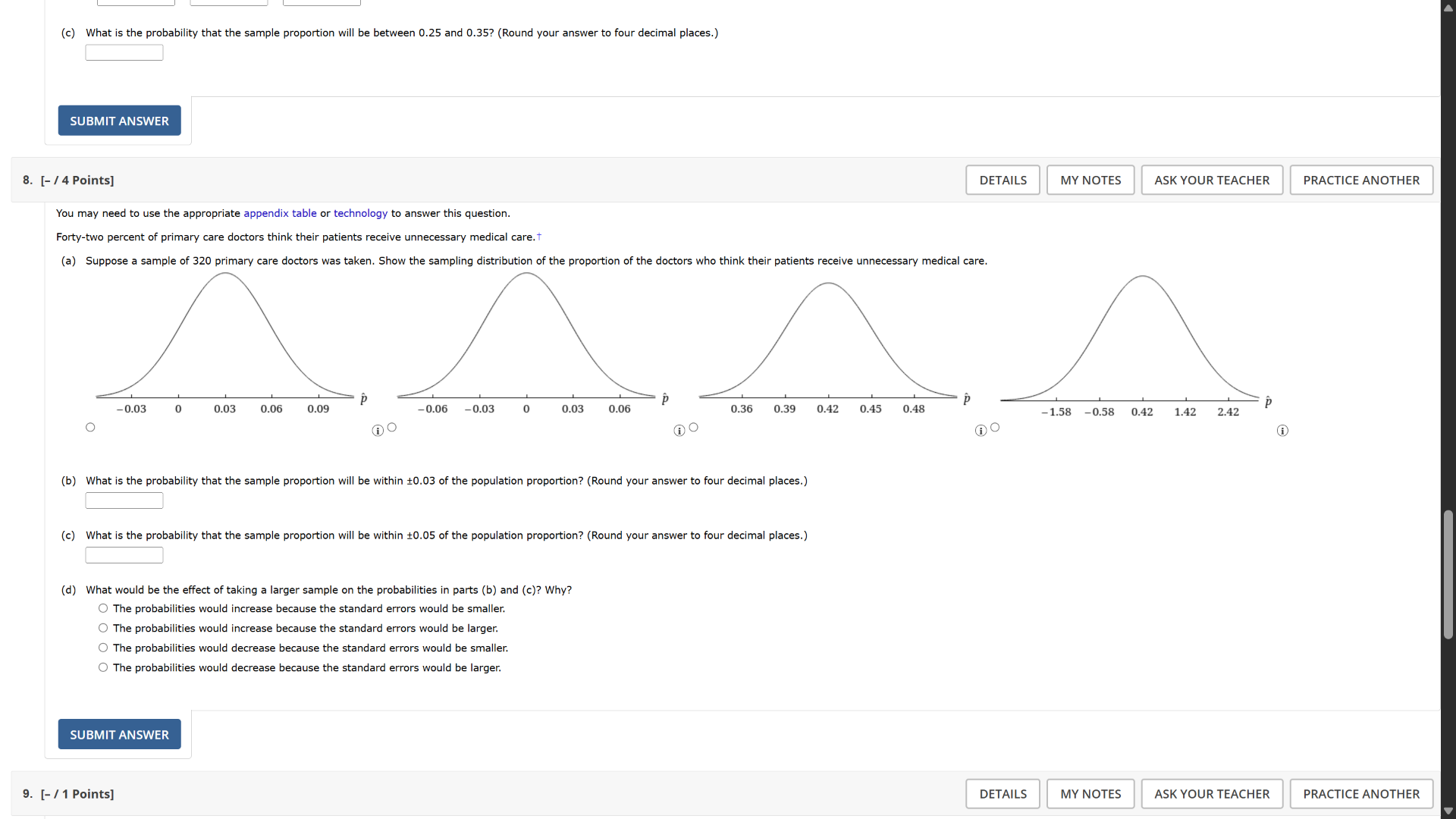
(c) what is the probability that the sample proportion will be between 0.25 and 0.35? (round your answer to four decimal places.) submit answer 8. - / 4 points you may need to use the appropriate appendix table or technology to answer this question. forty - two percent of primary care doctors think their patients receive unnecessary medical care. (a) suppose a sample of 320 primary care doctors was taken. show the sampling distribution of the proportion of the doctors who think their patients receive unnecessary medical care. (b) what is the probability that the sample proportion will be within ±0.03 of the population proportion? (round your answer to four decimal places.) (c) what is the probability that the sample proportion will be within ±0.05 of the population proportion? (round your answer to four decimal places.) (d) what would be the effect of taking a larger sample on the probabilities in parts (b) and (c)? why? the probabilities would increase because the standard errors would be smaller. the probabilities would increase because the standard errors would be larger. the probabilities would decrease because the standard errors would be smaller. the probabilities would decrease because the standard errors would be larger. submit answer 9. - / 1 points

Explanation:

Part (a)

To determine the sampling distribution of the sample proportion \(\hat{p}\), we use the properties of the sampling distribution of a proportion.

• The population proportion \(p = 0.42\) (since 42% of primary care doctors think their patients receive unnecessary medical care).
• The sample size \(n = 320\).

For the sampling distribution of \(\hat{p}\):

1. Mean: The mean of the sampling distribution of \(\hat{p}\) is equal to the population proportion \(p\). Thus, \(\mu_{\hat{p}} = p = 0.42\).
2. Standard Error (SE): The standard error of the sampling distribution of \(\hat{p}\) is calculated as:

\[
SE = \sqrt{\frac{p(1 - p)}{n}}
\]
Substituting \(p = 0.42\) and \(n = 320\):
\[
SE = \sqrt{\frac{0.42(1 - 0.42)}{320}} = \sqrt{\frac{0.42 \times 0.58}{320}} \approx \sqrt{\frac{0.2436}{320}} \approx \sqrt{0.00076125} \approx 0.0276
\]

The sampling distribution of \(\hat{p}\) is approximately normal (by the Central Limit Theorem, since \(np = 320 \times 0.42 = 134.4 \geq 5\) and \(n(1 - p) = 320 \times 0.58 = 185.6 \geq 5\)) with mean \(0.42\) and standard error \(\approx 0.0276\).

Part (b)

We need to find \(P(0.42 - 0.03 \leq \hat{p} \leq 0.42 + 0.03) = P(0.39 \leq \hat{p} \leq 0.45)\).

First, calculate the z-scores for \(\hat{p} = 0.39\) and \(\hat{p} = 0.45\):

• For \(\hat{p} = 0.39\):

\[
z_1 = \frac{0.39 - 0.42}{0.0276} \approx \frac{-0.03}{0.0276} \approx -1.09
\]

• For \(\hat{p} = 0.45\):

\[
z_2 = \frac{0.45 - 0.42}{0.0276} \approx \frac{0.03}{0.0276} \approx 1.09
\]

Using the standard normal table (or technology), we find:

• \(P(Z \leq -1.09) \approx 0.1379\)
• \(P(Z \leq 1.09) \approx 0.8621\)

Thus, the probability is:
\[
P(-1.09 \leq Z \leq 1.09) = P(Z \leq 1.09) - P(Z \leq -1.09) \approx 0.8621 - 0.1379 = 0.7242
\]

Part (c)

We need to find \(P(0.42 - 0.05 \leq \hat{p} \leq 0.42 + 0.05) = P(0.37 \leq \hat{p} \leq 0.47)\).

Calculate the z-scores for \(\hat{p} = 0.37\) and \(\hat{p} = 0.47\):

• For \(\hat{p} = 0.37\):

\[
z_1 = \frac{0.37 - 0.42}{0.0276} \approx \frac{-0.05}{0.0276} \approx -1.81
\]

• For \(\hat{p} = 0.47\):

\[
z_2 = \frac{0.47 - 0.42}{0.0276} \approx \frac{0.05}{0.0276} \approx 1.81
\]

Using the standard normal table (or technology), we find:

• \(P(Z \leq -1.81) \approx 0.0351\)
• \(P(Z \leq 1.81) \approx 0.9649\)

Thus, the probability is:
\[
P(-1.81 \leq Z \leq 1.81) = P(Z \leq 1.81) - P(Z \leq -1.81) \approx 0.9649 - 0.0351 = 0.9298
\]

Part (d)

The standard error of the sampling distribution of \(\hat{p}\) is \(\sqrt{\frac{p(1 - p)}{n}}\). As the sample size \(n\) increases, the standard error decreases (since \(n\) is in the denominator). A smaller standard error means the sampling distribution becomes narrower, so the probability that \(\hat{p}\) is within a fixed range of \(p\) (e.g., \(\pm 0.03\) or \(\pm 0.05\)) increases (because the interval around \(p\) covers more of the narrower distribution).

Thus, the correct option is:
The probabilities would increase because the standard errors would be smaller.

Final Answers

(a) Sampling distribution: Normal with \(\mu_{\hat{p}} = 0.42\) and \(SE \approx 0.0276\).
(b) \(\boldsymbol{0.7242}\)
(c) \(\boldsymbol{0.9298}\)
(d) The probabilities would increase because the standard errors would be smaller.

Answer:

Part (a)

To determine the sampling distribution of the sample proportion \(\hat{p}\), we use the properties of the sampling distribution of a proportion.

• The population proportion \(p = 0.42\) (since 42% of primary care doctors think their patients receive unnecessary medical care).
• The sample size \(n = 320\).

For the sampling distribution of \(\hat{p}\):

1. Mean: The mean of the sampling distribution of \(\hat{p}\) is equal to the population proportion \(p\). Thus, \(\mu_{\hat{p}} = p = 0.42\).
2. Standard Error (SE): The standard error of the sampling distribution of \(\hat{p}\) is calculated as:

\[
SE = \sqrt{\frac{p(1 - p)}{n}}
\]
Substituting \(p = 0.42\) and \(n = 320\):
\[
SE = \sqrt{\frac{0.42(1 - 0.42)}{320}} = \sqrt{\frac{0.42 \times 0.58}{320}} \approx \sqrt{\frac{0.2436}{320}} \approx \sqrt{0.00076125} \approx 0.0276
\]

The sampling distribution of \(\hat{p}\) is approximately normal (by the Central Limit Theorem, since \(np = 320 \times 0.42 = 134.4 \geq 5\) and \(n(1 - p) = 320 \times 0.58 = 185.6 \geq 5\)) with mean \(0.42\) and standard error \(\approx 0.0276\).

Part (b)

We need to find \(P(0.42 - 0.03 \leq \hat{p} \leq 0.42 + 0.03) = P(0.39 \leq \hat{p} \leq 0.45)\).

First, calculate the z-scores for \(\hat{p} = 0.39\) and \(\hat{p} = 0.45\):

• For \(\hat{p} = 0.39\):

\[
z_1 = \frac{0.39 - 0.42}{0.0276} \approx \frac{-0.03}{0.0276} \approx -1.09
\]

• For \(\hat{p} = 0.45\):

\[
z_2 = \frac{0.45 - 0.42}{0.0276} \approx \frac{0.03}{0.0276} \approx 1.09
\]

Using the standard normal table (or technology), we find:

• \(P(Z \leq -1.09) \approx 0.1379\)
• \(P(Z \leq 1.09) \approx 0.8621\)

Thus, the probability is:
\[
P(-1.09 \leq Z \leq 1.09) = P(Z \leq 1.09) - P(Z \leq -1.09) \approx 0.8621 - 0.1379 = 0.7242
\]

Part (c)

We need to find \(P(0.42 - 0.05 \leq \hat{p} \leq 0.42 + 0.05) = P(0.37 \leq \hat{p} \leq 0.47)\).

Calculate the z-scores for \(\hat{p} = 0.37\) and \(\hat{p} = 0.47\):

• For \(\hat{p} = 0.37\):

\[
z_1 = \frac{0.37 - 0.42}{0.0276} \approx \frac{-0.05}{0.0276} \approx -1.81
\]

• For \(\hat{p} = 0.47\):

\[
z_2 = \frac{0.47 - 0.42}{0.0276} \approx \frac{0.05}{0.0276} \approx 1.81
\]

Using the standard normal table (or technology), we find:

• \(P(Z \leq -1.81) \approx 0.0351\)
• \(P(Z \leq 1.81) \approx 0.9649\)

Thus, the probability is:
\[
P(-1.81 \leq Z \leq 1.81) = P(Z \leq 1.81) - P(Z \leq -1.81) \approx 0.9649 - 0.0351 = 0.9298
\]

Part (d)

The standard error of the sampling distribution of \(\hat{p}\) is \(\sqrt{\frac{p(1 - p)}{n}}\). As the sample size \(n\) increases, the standard error decreases (since \(n\) is in the denominator). A smaller standard error means the sampling distribution becomes narrower, so the probability that \(\hat{p}\) is within a fixed range of \(p\) (e.g., \(\pm 0.03\) or \(\pm 0.05\)) increases (because the interval around \(p\) covers more of the narrower distribution).

Thus, the correct option is:
The probabilities would increase because the standard errors would be smaller.

Final Answers

(a) Sampling distribution: Normal with \(\mu_{\hat{p}} = 0.42\) and \(SE \approx 0.0276\).
(b) \(\boldsymbol{0.7242}\)
(c) \(\boldsymbol{0.9298}\)
(d) The probabilities would increase because the standard errors would be smaller.