Question

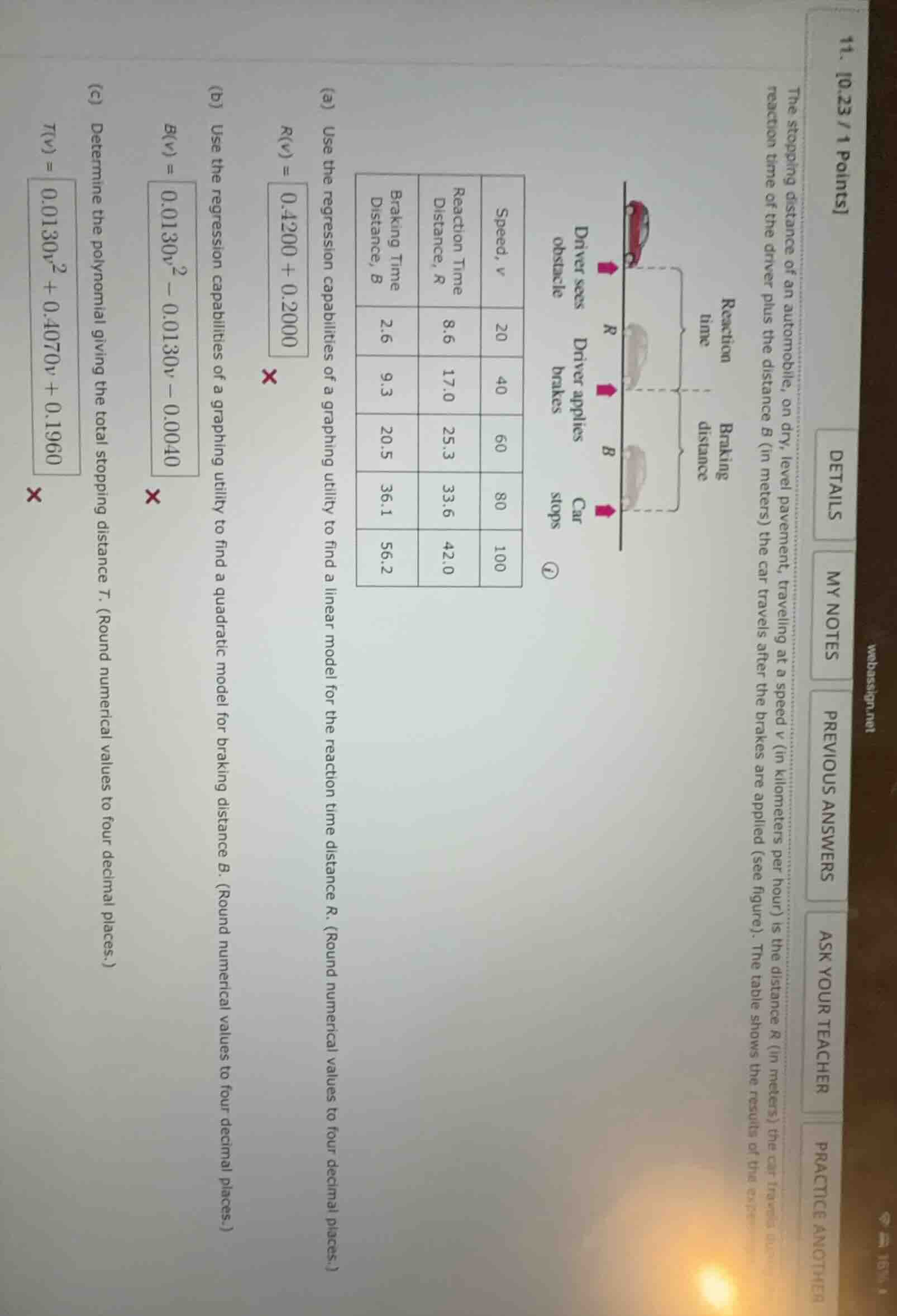
1. 0.23 / 1 points details my notes previous answers ask your teacher practice another the stopping distance of an automobile, on dry, level pavement, travelling at a speed ( v ) (in kilometers per hour) is the distance ( r ) (in meters) the car travels during reaction time of the driver plus the distance ( b ) (in meters) the car travels after the brakes are applied (see figure). the table shows the results of the experiments. (a) use the regression capabilities of a graphing utility to find a linear model for the reaction time distance ( r ). (round numerical values to four decimal places.) ( r(v) = 0.4200 + 0.2000 ) (b) use the regression capabilities of a graphing utility to find a quadratic model for braking distance ( b ). (round numerical values to four decimal places.) ( b(v) = 0.0130v^2 - 0.0130v - 0.0040 ) (c) determine the polynomial giving the total stopping distance ( t ). (round numerical values to four decimal places.) ( t(v) = 0.0130v^2 + 0.4070v + 0.1960 )

Explanation:

Part (a): Linear Model for Reaction Distance \( R(v) \)

Step 1: Identify Data Points

We have the following data points for speed \( v \) (in km/h) and reaction distance \( R \) (in meters):
\( (20, 8.6) \), \( (40, 17.0) \), \( (60, 25.3) \), \( (80, 33.6) \), \( (100, 42.0) \).

Step 2: Use Linear Regression

A linear model has the form \( R(v) = av + b \). Using a graphing utility or calculator for linear regression on the data:

• Input the \( v \)-values (20, 40, 60, 80, 100) and \( R \)-values (8.6, 17.0, 25.3, 33.6, 42.0).
• The regression output gives \( a \approx 0.4200 \) and \( b \approx 0.2000 \) (rounded to four decimal places).

Part (b): Quadratic Model for Braking Distance \( B(v) \)

Step 1: Identify Data Points

Data points for speed \( v \) and braking distance \( B \):
\( (20, 2.6) \), \( (40, 9.3) \), \( (60, 20.5) \), \( (80, 36.1) \), \( (100, 56.2) \).

Step 2: Use Quadratic Regression

A quadratic model has the form \( B(v) = av^2 + bv + c \). Using a graphing utility for quadratic regression:

• Input \( v \)-values (20, 40, 60, 80, 100) and \( B \)-values (2.6, 9.3, 20.5, 36.1, 56.2).
• The regression output (rounded to four decimal places) gives \( a \approx 0.0130 \), \( b \approx -0.0130 \), \( c \approx -0.0040 \). Thus, \( B(v) = 0.0130v^2 - 0.0130v - 0.0040 \).

Part (c): Total Stopping Distance \( T(v) \)

Step 1: Define Total Distance

Total stopping distance \( T(v) = R(v) + B(v) \).

Step 2: Substitute Models

From part (a): \( R(v) = 0.4200v + 0.2000 \)
From part (b): \( B(v) = 0.0130v^2 - 0.0130v - 0.0040 \)

Add them:
\( T(v) = (0.0130v^2 - 0.0130v - 0.0040) + (0.4200v + 0.2000) \)
Simplify:
\( T(v) = 0.0130v^2 + ( -0.0130v + 0.4200v ) + ( -0.0040 + 0.2000 ) \)
\( T(v) = 0.0130v^2 + 0.4070v + 0.1960 \)

Answer:

s:
(a) \( \boldsymbol{R(v) = 0.4200v + 0.2000} \)
(b) \( \boldsymbol{B(v) = 0.0130v^2 - 0.0130v - 0.0040} \)
(c) \( \boldsymbol{T(v) = 0.0130v^2 + 0.4070v + 0.1960} \)