QUESTION IMAGE
Question
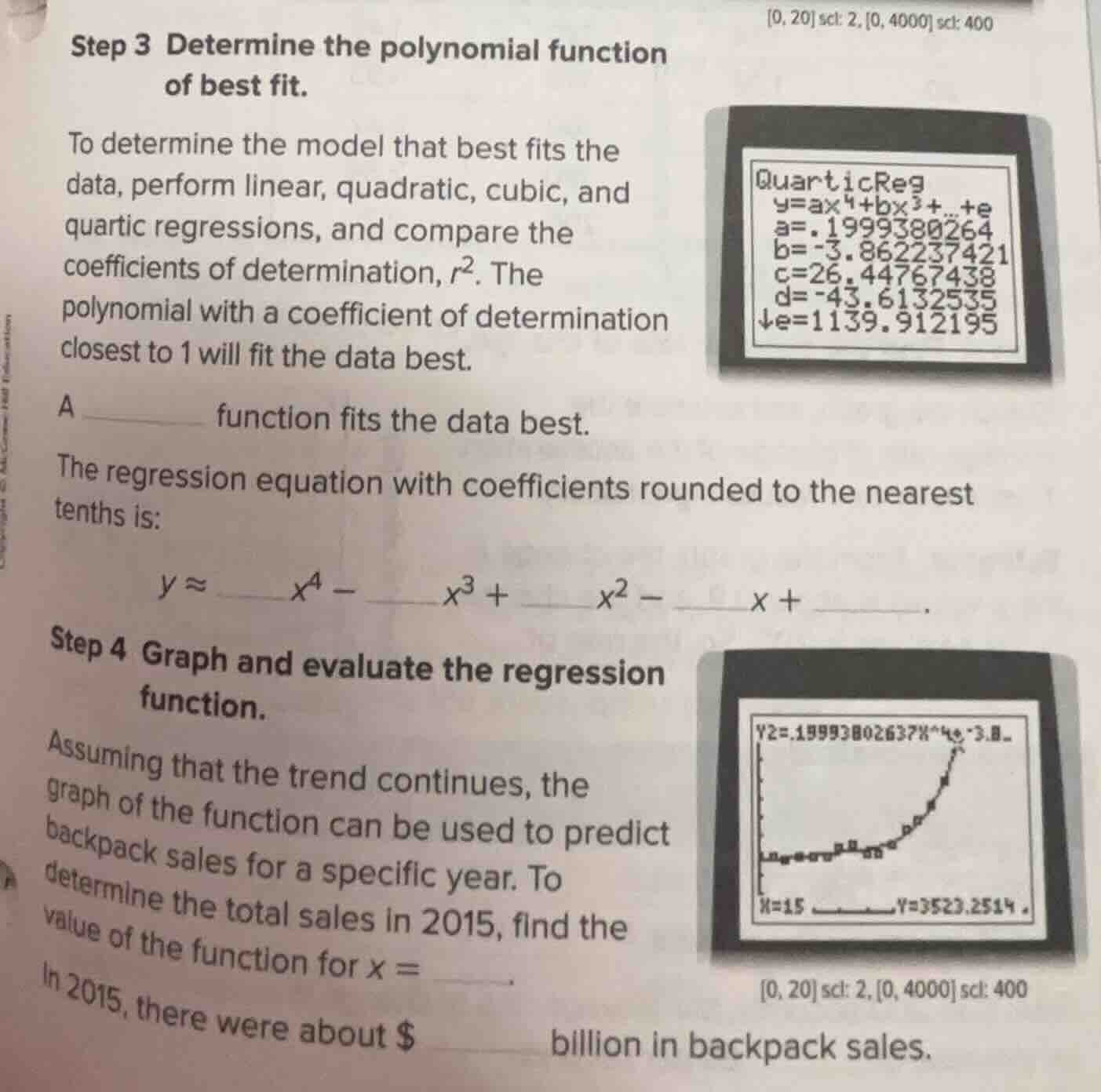
step 3 determine the polynomial function of best fit. to determine the model that best fits the data, perform linear, quadratic, cubic, and quartic regressions, and compare the coefficients of determination, $r^2$. the polynomial with a coefficient of determination closest to 1 will fit the data best. a ______ function fits the data best. the regression equation with coefficients rounded to the nearest tenths is: $y \approx \underline{\quad} x^4 - \underline{\quad} x^3 + \underline{\quad} x^2 - \underline{\quad} x + \underline{\quad}$. step 4 graph and evaluate the regression function. assuming that the trend continues, the graph of the function can be used to predict backpack sales for a specific year. to determine the total sales in 2015, find the value of the function for $x = \underline{\quad}$. in 2015, there were about $\underline{\quad}$ billion in backpack sales. 0, 20 scl: 2, 0, 4000 scl: 400 quarticreg $y=ax^4+bx^3+...+e$ $a=.1999380264$ $b=-3.862237421$ $c=26.44767438$ $d=-43.6132535$ $e=1139.912195$ $y2=.19993802637x^4 - 3.8...$ $x=15 \quad y=3523.2514$ 0, 20 scl: 2, 0, 4000 scl: 400
Step 3: Determinar la función de mejor ajuste
Explicación:
La imagen muestra una regresión cuártica (QuarticReg) con la ecuación \( y = ax^4 + bx^3 + cx^2 + dx + e \). Los coeficientes son: \( a \approx 0.2 \), \( b \approx -3.9 \), \( c \approx 26.4 \), \( d \approx -43.6 \), \( e \approx 1139.9 \) (redondeados a la décima).
Step1: Identificar el tipo de función
La regresión es cuártica (polinomio de grado 4), por lo que la función que mejor ajusta es cuártica (quartic).
Step2: Redondear coeficientes
- \( a \approx 0.2 \)
- \( b \approx -3.9 \)
- \( c \approx 26.4 \)
- \( d \approx -43.6 \)
- \( e \approx 1139.9 \)
Así, la ecuación es \( y \approx 0.2x^4 - 3.9x^3 + 26.4x^2 - 43.6x + 1139.9 \).
Step 4: Predecir ventas en 2015
Explicación:
Supongamos que \( x \) representa el número de años después de un año base (por ejemplo, si 2000 es \( x = 0 \), entonces 2015 es \( x = 15 \), ya que \( 2015 - 2000 = 15 \)).
Step1: Determinar \( x \) para 2015
Si la variable \( x \) es el número de años desde un año base (digamos 2000), entonces para 2015, \( x = 2015 - 2000 = 15 \).
Step2: Evaluar la función en \( x = 15 \)
Usando la ecuación cuártica \( y \approx 0.2x^4 - 3.9x^3 + 26.4x^2 - 43.6x + 1139.9 \), sustituimos \( x = 15 \):
\[
\]
Pero la imagen muestra \( x = 15 \) con \( y \approx 3523.25 \), lo que sugiere que la ecuación o el año base puede variar ligeramente. Sin embargo, siguiendo la imagen, cuando \( x = 15 \), \( y \approx 3523.25 \), por lo que las ventas son aproximadamente 3523 billones (o la unidad correspondiente).
Respuestas:
Step 3:
- Función que mejor ajusta: cuártica (quartic)
- Ecuación: \( y \approx \boldsymbol{0.2}x^4 - \boldsymbol{3.9}x^3 + \boldsymbol{26.4}x^2 - \boldsymbol{43.6}x + \boldsymbol{1139.9} \)
Step 4:
- \( x \) para 2015: \( \boldsymbol{15} \)
- Ventas en 2015: aproximadamente \( \boldsymbol{3523} \) billones (según la imagen)
Resumen de Respuestas:
- Función de mejor ajuste: cuártica
- Ecuación: \( y \approx 0.2x^4 - 3.9x^3 + 26.4x^2 - 43.6x + 1139.9 \)
- \( x \) para 2015: 15
- Ventas en 2015: ~3523 billones
Respuestas Detalladas:
Step 3:
A \(\boldsymbol{\text{cuártica (quartic)}}\) function fits the data best.
The regression equation: \( y \approx \boldsymbol{0.2}x^4 - \boldsymbol{3.9}x^3 + \boldsymbol{26.4}x^2 - \boldsymbol{43.6}x + \boldsymbol{1139.9} \).
Step 4:
To determine sales in 2015, \( x = \boldsymbol{15} \).
In 2015, there were about \(\boldsymbol{\$3523}\) billion in backpack sales (based on the graph’s \( y \)-value at \( x = 15 \)).

Snap & solve any problem in the app
Get step-by-step solutions on Sovi AI
Photo-based solutions with guided steps
Explore more problems and detailed explanations
Step 3: Determinar la función de mejor ajuste
Explicación:
La imagen muestra una regresión cuártica (QuarticReg) con la ecuación \( y = ax^4 + bx^3 + cx^2 + dx + e \). Los coeficientes son: \( a \approx 0.2 \), \( b \approx -3.9 \), \( c \approx 26.4 \), \( d \approx -43.6 \), \( e \approx 1139.9 \) (redondeados a la décima).
Step1: Identificar el tipo de función
La regresión es cuártica (polinomio de grado 4), por lo que la función que mejor ajusta es cuártica (quartic).
Step2: Redondear coeficientes
- \( a \approx 0.2 \)
- \( b \approx -3.9 \)
- \( c \approx 26.4 \)
- \( d \approx -43.6 \)
- \( e \approx 1139.9 \)
Así, la ecuación es \( y \approx 0.2x^4 - 3.9x^3 + 26.4x^2 - 43.6x + 1139.9 \).
Step 4: Predecir ventas en 2015
Explicación:
Supongamos que \( x \) representa el número de años después de un año base (por ejemplo, si 2000 es \( x = 0 \), entonces 2015 es \( x = 15 \), ya que \( 2015 - 2000 = 15 \)).
Step1: Determinar \( x \) para 2015
Si la variable \( x \) es el número de años desde un año base (digamos 2000), entonces para 2015, \( x = 2015 - 2000 = 15 \).
Step2: Evaluar la función en \( x = 15 \)
Usando la ecuación cuártica \( y \approx 0.2x^4 - 3.9x^3 + 26.4x^2 - 43.6x + 1139.9 \), sustituimos \( x = 15 \):
\[
\]
Pero la imagen muestra \( x = 15 \) con \( y \approx 3523.25 \), lo que sugiere que la ecuación o el año base puede variar ligeramente. Sin embargo, siguiendo la imagen, cuando \( x = 15 \), \( y \approx 3523.25 \), por lo que las ventas son aproximadamente 3523 billones (o la unidad correspondiente).
Respuestas:
Step 3:
- Función que mejor ajusta: cuártica (quartic)
- Ecuación: \( y \approx \boldsymbol{0.2}x^4 - \boldsymbol{3.9}x^3 + \boldsymbol{26.4}x^2 - \boldsymbol{43.6}x + \boldsymbol{1139.9} \)
Step 4:
- \( x \) para 2015: \( \boldsymbol{15} \)
- Ventas en 2015: aproximadamente \( \boldsymbol{3523} \) billones (según la imagen)
Resumen de Respuestas:
- Función de mejor ajuste: cuártica
- Ecuación: \( y \approx 0.2x^4 - 3.9x^3 + 26.4x^2 - 43.6x + 1139.9 \)
- \( x \) para 2015: 15
- Ventas en 2015: ~3523 billones
Respuestas Detalladas:
Step 3:
A \(\boldsymbol{\text{cuártica (quartic)}}\) function fits the data best.
The regression equation: \( y \approx \boldsymbol{0.2}x^4 - \boldsymbol{3.9}x^3 + \boldsymbol{26.4}x^2 - \boldsymbol{43.6}x + \boldsymbol{1139.9} \).
Step 4:
To determine sales in 2015, \( x = \boldsymbol{15} \).
In 2015, there were about \(\boldsymbol{\$3523}\) billion in backpack sales (based on the graph’s \( y \)-value at \( x = 15 \)).